Quantum Oracle Circuits and the Christmas Tree Pattern
Blog article by Mathias Soeken from December 19, 2018, written for the
Q# Advent Calendar
licensed under
CC-BY 4.0
Donald E. Knuth introduced the Christmas tree pattern sixteen years ago in his ninth annual Christmas tree lecture at Stanford University, and he has made it part of Section 7.2.1.6 in his famous multi-volume work The Art of Computer Programming. The recursive definition of the Christmas tree pattern goes as follows. The Christmas tree pattern of order \(1\) is a single row ‘\(0 \; 1\)’. One obtains the Christmas tree pattern of order \(n+1\) by taking each row of elements ‘\(\sigma_1\; \sigma_2\; \ldots \sigma_s\)’ in the pattern of order \(n\) and replace it by the following two rows: $$ \begin{array}{ccccc} & \sigma_20 & \ldots & \sigma_s0 & \\ \sigma_10 & \sigma_11 & \ldots & \sigma_{s-1}1 & \sigma_s1\end{array} $$ The first of these two rows is omitted when \(s = 1\). The Christmas tree pattern of orders \(2\) to \(4\) are:
| $$ \begin{array}{ccc} & 10 & \\ 00 & 01 & 11 \end{array} $$ | $$ \begin{array}{ccc} & 100 & 101 & \\ & 010 & 110 & \\ 000 & 001 & 011 & 111 \end{array} $$ |
$$ \begin{array}{ccc} & & 1010 & & \\ & 1000 & 1001 & 1011 & \\ & & 1100 & & \\ & 0100 & 0101 & 1101 & \\ & 0010 & 0110 & 1110 & \\ 0000 & 0001 & 0011 & 0111 & 1111 \end{array} $$
|
Knuth describes many interesting properties of this pattern in his book. But one of the most apparent ones is that the pattern of order \(n\) contains all \(2^n\) bitstrings of length \(n\), grouped into \(n+1\) columns according to the number of \(1\)’s in the bitstring. For now the Christmas tree pattern is visualized in green, but because it's Christmas, we should decorate the tree! In this blog article, I will use the implementation complexity of quantum oracles to decide which decoration to put.
The Christmas tree pattern of order \(n\) can be used to visualize all the input combinations of an \(n\)-variable Boolean function. Moreover, the Christmas tree pattern of order \(2^n\) can be used to either visualize all the input combinations of an \(2^n\)-variable Boolean function, but also to visualize all \(n\)-variable Boolean functions themselves. For example, the Christmas tree pattern of order \(4\) contains all 16 2-variable Boolean functions.
Quantum oracles
The central quantum operations in this blog article are quantum oracle funtions $$ U_f : |x_1x_2\ldots x_n\rangle|y\rangle \mapsto |x_1x_2\ldots x_n\rangle|y \oplus f(x_1, x_2, \dots, x_n)\rangle $$ implemented in terms of quantum circuits using the Hadamard gate, CNOT gates, and arbitrary Z-rotation gates. The following general circuit construction is based on the work by Schuch and Siewert and Welch et al, and here illustrated for a generic 2-variable Boolean oracle function \(f(x_1, x_2)\).
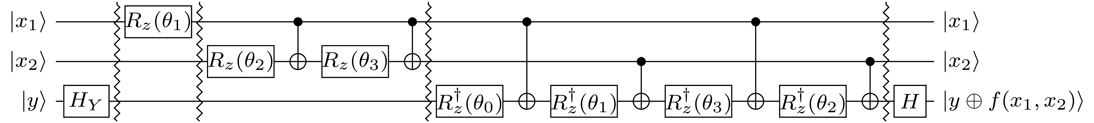
The nice property about this construction is that it can be used to find a circuit for each of the 16 possible functions \(f\), by only changing the values for the rotation angles \(\theta_0, \dots, \theta_3\). Before we discuss how to determine these values, I'd like to point out the recursive structure of the construction: If we leave out the surrounding Hadamard gate \(H\) and \(Y\)-Hadamard gate \(H_Y = SH\), there are three compartments \(1, 2, 3\), separated by barrier lines, one compartment for each qubit. Let's for simplicity define \(x_3 = y\). Then, the CNOT gates in compartment \(i\) prepare all linear functions that include \(x_i\) but do not include a variable with a larger index. All CNOT gates in compartment \(i\) have the target on qubit \(i\) and controls on qubits with a smaller index. The first compartment does not need a CNOT gate, since it has \(x_1\) on the first qubit. The second compartment computes \(x_2 \oplus x_1\), and then applies the CNOT gate again to revert the state of the second qubit back to \(x_2\). Finally, CNOT gates in the third compartment are used to compute \(x_3 \oplus x_1\), \(x_3 \oplus x_2 \oplus x_1\), and \(x_3 \oplus x_2\). The controls of the CNOT gates are chosen such that the control patterns are generated using a Gray code sequence—that minimizes the number of CNOT gates! Extending this circuit to a 4-qubit quantum circuit implementing oracles with 3 input variables is easy: one just needs to add a fourth compartment with 8 CNOT gates that add all linear functions that include \(x_4\).
That explains the CNOT gates, but what about the angles \(\theta_j\)? These can be computed from the spectral coefficients \(s_j\) of the oracle function \(f(x_1, x_2)\). We obtain the spectral coefficients by applying the Hadamard transform \(H_2 = \left(\begin{smallmatrix} 1 & \hfil 1 \\ 1 & -1 \end{smallmatrix}\right) \otimes \left(\begin{smallmatrix} 1 & \hfil 1 \\ 1 & -1 \end{smallmatrix}\right)\) to the truth table of \(f(x_1, x_2)\) in \(\{-1,1\}\)-encoding. This encoding simply replaces every 0 with a 1, and every 1 with a -1. In other words, we have \(f_{x_2x_1} = (-1)^{f(x_1, x_2)}\).
$$ \left[ \begin{array}{rrrr} 1 & 1 & 1 & 1 \\ 1 & -1 & 1 & -1 \\ 1 & 1 & -1 & -1 \\ 1 & -1 & -1 & 1 \end{array} \right] \left[ \begin{array}{c} f_{00} \\ f_{01} \\ f_{10} \\ f_{11} \\ \end{array} \right] = \left[ \begin{array}{c} s_0 \\ s_1 \\ s_2 \\ s_3 \\ \end{array} \right] $$
By setting \(\theta_j = \frac{\pi s_j}{2^3}\), the above circuit implements the oracle function. For example, if \(f(x_1, x_2) = x_1 \land x_2\), then \(s_0 = s_1 = s_2 = 2\), and \(s_3 = -2\), and therefore \(\theta_0 = \theta_1 = \theta_2 = \frac{\pi}{4}\) and \(\theta_3 = -\frac{\pi}{4}\), hence, resulting in the well-known circuit construction with 7 \(T\) and \(T^\dagger\) gates. (Side remark: If \(|y\rangle = |0\rangle\), then the circuit can be simplified by removing all but the last compartment. This generalizes Craig Gidney's construction for the Toffoli gate.)
Implementation in Q#
I have
implemented the above algorithm for oracle synthesis
in Q#.
The complete source code is on Github, but the main operation is printed below.
The first two lines in the operation
Oracle
compute the \(\{1,-1\}\) value vector for the oracle function,
as well as the spectral coefficients by applying the Hadamard transform in
an efficient way using Yates's method.
The
Extend
method extends the spectral coefficients by their inverses as described in the example above.
// First in tuple is value in GrayCode sequence
// Second in tuple is position to change in current value to get next one
//   Ex: GrayCode(2) = [(0, 0);(1, 1);(3, 0);(2, 1)]
function GrayCode(n : Int) : (Int, Int)[] {
  // ...
}

operation Oracle(func : Int, controls : Qubit[], target : Qubit) : Unit {
  let vars = Length(controls);
  let table = Encode(TruthTable(func, vars));
  let spectrum = Extend(FastHadamardTransform(table));

  let qubits = controls + [target];

  HY(target);

  for (i in 0..vars) {
    let start = 1 <<< i;
    let code = GrayCode(i);
    for (j in 0..Length(code) - 1) {
      let (offset, ctrl) = code[j];
      RFrac(PauliZ, -spectrum[start + offset], vars + 2, qubits[i]);
      if (i != 0) {
        CNOT(qubits[ctrl], qubits[i]);
      }
    }
  }

  H(target);
}
The
RFrac
operation implements the rotation gates, and the
CNOT
operation implements the CNOT gate, which does not need to be applied in the first compartment.
Coloring the Christmas Tree
Let's apply the above oracle synthesis to all 3-input Boolean functions. Of course, each of the 256 functions has a different spectrum with 8 coefficients. But if we consider the absolute values of the coefficients and sort them, then all functions will fall into one of the following 3 classes:
$$ 0\, 0\, 0\, 0\, 0\, 0\, 0\, 8, \quad 0\, 0\, 0\, 0\, 4\, 4\, 4\, 4, \quad 2\, 2\, 2\, 2\, 2\, 2\, 2\, 6 $$
The most narrow rotation angle in the first class is an \(S\) gate, in the second class a \(T\) gate, and in the third class a \(\sqrt{T}\) gate. Let's decorate the Christmas tree of order 8, by coloring each function from the first class in green, from the second class in yellow, and from the third class in red. Merry Christmas!
| 10101010 | ||||||||
| 10101000 | 10101001 | 10101011 | ||||||
| 10101100 | ||||||||
| 10100100 | 10100101 | 10101101 | ||||||
| 10100010 | 10100110 | 10101110 | ||||||
| 10100000 | 10100001 | 10100011 | 10100111 | 10101111 | ||||
| 10110010 | ||||||||
| 10110000 | 10110001 | 10110011 | ||||||
| 10110100 | ||||||||
| 10010100 | 10010101 | 10110101 | ||||||
| 10010010 | 10010110 | 10110110 | ||||||
| 10010000 | 10010001 | 10010011 | 10010111 | 10110111 | ||||
| 10111000 | ||||||||
| 10011000 | 10011001 | 10111001 | ||||||
| 10001010 | 10011010 | 10111010 | ||||||
| 10001000 | 10001001 | 10001011 | 10011011 | 10111011 | ||||
| 10001100 | 10011100 | 10111100 | ||||||
| 10000100 | 10000101 | 10001101 | 10011101 | 10111101 | ||||
| 10000010 | 10000110 | 10001110 | 10011110 | 10111110 | ||||
| 10000000 | 10000001 | 10000011 | 10000111 | 10001111 | 10011111 | 10111111 | ||
| 11001010 | ||||||||
| 11001000 | 11001001 | 11001011 | ||||||
| 11001100 | ||||||||
| 11000100 | 11000101 | 11001101 | ||||||
| 11000010 | 11000110 | 11001110 | ||||||
| 11000000 | 11000001 | 11000011 | 11000111 | 11001111 | ||||
| 11010010 | ||||||||
| 11010000 | 11010001 | 11010011 | ||||||
| 11010100 | ||||||||
| 01010100 | 01010101 | 11010101 | ||||||
| 01010010 | 01010110 | 11010110 | ||||||
| 01010000 | 01010001 | 01010011 | 01010111 | 11010111 | ||||
| 11011000 | ||||||||
| 01011000 | 01011001 | 11011001 | ||||||
| 01001010 | 01011010 | 11011010 | ||||||
| 01001000 | 01001001 | 01001011 | 01011011 | 11011011 | ||||
| 01001100 | 01011100 | 11011100 | ||||||
| 01000100 | 01000101 | 01001101 | 01011101 | 11011101 | ||||
| 01000010 | 01000110 | 01001110 | 01011110 | 11011110 | ||||
| 01000000 | 01000001 | 01000011 | 01000111 | 01001111 | 01011111 | 11011111 | ||
| 11100010 | ||||||||
| 11100000 | 11100001 | 11100011 | ||||||
| 11100100 | ||||||||
| 01100100 | 01100101 | 11100101 | ||||||
| 01100010 | 01100110 | 11100110 | ||||||
| 01100000 | 01100001 | 01100011 | 01100111 | 11100111 | ||||
| 11101000 | ||||||||
| 01101000 | 01101001 | 11101001 | ||||||
| 00101010 | 01101010 | 11101010 | ||||||
| 00101000 | 00101001 | 00101011 | 01101011 | 11101011 | ||||
| 00101100 | 01101100 | 11101100 | ||||||
| 00100100 | 00100101 | 00101101 | 01101101 | 11101101 | ||||
| 00100010 | 00100110 | 00101110 | 01101110 | 11101110 | ||||
| 00100000 | 00100001 | 00100011 | 00100111 | 00101111 | 01101111 | 11101111 | ||
| 11110000 | ||||||||
| 01110000 | 01110001 | 11110001 | ||||||
| 00110010 | 01110010 | 11110010 | ||||||
| 00110000 | 00110001 | 00110011 | 01110011 | 11110011 | ||||
| 00110100 | 01110100 | 11110100 | ||||||
| 00010100 | 00010101 | 00110101 | 01110101 | 11110101 | ||||
| 00010010 | 00010110 | 00110110 | 01110110 | 11110110 | ||||
| 00010000 | 00010001 | 00010011 | 00010111 | 00110111 | 01110111 | 11110111 | ||
| 00111000 | 01111000 | 11111000 | ||||||
| 00011000 | 00011001 | 00111001 | 01111001 | 11111001 | ||||
| 00001010 | 00011010 | 00111010 | 01111010 | 11111010 | ||||
| 00001000 | 00001001 | 00001011 | 00011011 | 00111011 | 01111011 | 11111011 | ||
| 00001100 | 00011100 | 00111100 | 01111100 | 11111100 | ||||
| 00000100 | 00000101 | 00001101 | 00011101 | 00111101 | 01111101 | 11111101 | ||
| 00000010 | 00000110 | 00001110 | 00011110 | 00111110 | 01111110 | 11111110 | ||
| 00000000 | 00000001 | 00000011 | 00000111 | 00001111 | 00011111 | 00111111 | 01111111 | 11111111 |
Appendix
Above, it is mentioned that the technique generalizes to Craig Gidney's construction for the Toffoli gate. The technique applies to all Boolean functions with \(n\) variables, but is illustrated for simplicity for \(n = 2\). If the target qubit is initialized to \(|0\rangle\), one only needs the last compartment, and can omit all other ones:
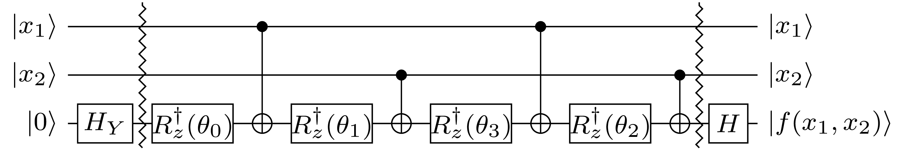
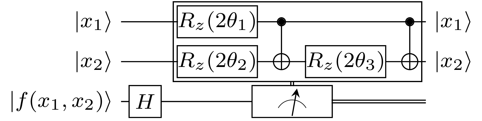
When uncomputing the oracle function, i.e., we expect that the ancilla qubit is restored to 0, one can use the following circuit which uses all but the last compartments from the circuit. Also, all angles are multiplied by two:
Both circuits can be implemented inside a single Q# operation using the
adjoint
keyword:
operation OracleAncilla(func : Int, controls : Qubit[], target : Qubit) : Unit {
  body (...) {
    let vars = Length(controls);
    let table = Encode(TruthTable(func, vars));
    let spectrum = Extend(FastHadamardTransform(table));

    HY(target);

    let code = GrayCode(vars);
    for (j in 0..Length(code) - 1) {
      let (offset, ctrl) = code[j];
      RFrac(PauliZ, spectrum[offset], vars + 2, target);
      CNOT(controls[ctrl], target);
    }

    H(target);
  }
  adjoint (...) {
    let vars = Length(controls);
    let table = Encode(TruthTable(func, vars));
    let spectrum = Extend(FastHadamardTransform(table));

    H(target);
    if (IsResultOne(M(target))) {
      for (i in 0..vars - 1) {
        let start = 1 <<< i;
        let code = GrayCode(i);
        for (j in 0..Length(code) - 1) {
          let (offset, ctrl) = code[j];
          RFrac(PauliZ, -spectrum[start + offset], vars + 1, controls[i]);
          if (i != 0) {
            CNOT(controls[ctrl], controls[i]);
          }
        }
      }
      Reset(target);
    }
  }
}